This vignette provides a reference workflow for functional enrichment analysis, building on our earlier guide for differential abundance analysis. We demonstrate how to use the R package clusterProfiler to test protein lists for enrichment of Gene Ontology (GO) terms, as well as other functional and disease-related annotations. The clusterProfiler package is well-documented in manuscripts (Xu et al. 2024; Wu et al. 2021) and other online resources1. Here we demonstrate a clusterProfiler workflow tailored to proteomics data acquired in our lab. The workflow can be adapted to more complex experimental designs.
Functional enrichment analysis can be approached in two main ways:
Over-Representation Analysis (ORA): Identifies functional terms (e.g., GO terms or pathways) that are over-represented in a predefined list of “significant” proteins (e.g. differentially expressed proteins) compared to a background “universe” (e.g. all proteins detected in an experiment). ORA is widely applicable to most experimental designs and is generally straightforward to interpret.
Gene Set Enrichment Analysis (GSEA): Ranks all proteins by a continuous value (e.g. fold-change or p-value) and identifies functional terms that are enriched towards the top or bottom of the ranked list. Unlike ORA, GSEA can detect more subtle, coordinated changes without requiring a hard threshold for “significance.” However, it requires an appropriate ranking metric to be available.
The statistical principles behind these approaches are described in many online resources, such as this video series.
How to follow this vignette
Copy the R code chunks and run them locally as you go through this document. You should already be familiar with R data.table and ggplot. The input file DAA_results.csv.gz is produced by the Differential abundance analysis tutorial. The source code for the whole document is accessible through the Code button in the top right.
1 Preparing the data
As an example, we analyse a simple proteomics experiment that compares protein abundances between two cell lines (SS6 and SS48). We start with a data table containing the log2 fold-changes (e.g. log2_FC_SS6vsSS48) and p-values (e.g. adj_p_value) derived from a differential protein expression analysis.
Code
# Load the required librarieslibrary(data.table); library(ggplot2); library(highcharter); library(DT); library(clusterProfiler); library(DOSE); library(ReactomePA); library(enrichplot); library(org.Hs.eg.db); library(patchwork)# Load the relevant columns from the differentical expression analysisDT <-fread("DAA_results.csv.gz", select =c("Protein_group", "gene_group", "Genes", "Protein_description", "log2_FC_SS6vsSS48", "adj_p_value"))# Print key columns of this tableDT[ 1:5 , .(Protein_group, gene_group, log2_FC_SS6vsSS48, adj_p_value)]
For this analysis, we define the target list as proteins upregulated by more than 1.5-fold in the SS6 cell line, with an adjusted p-value < 0.05 (n = 181). We identify proteins using the gene_group column, which contains UniProt gene-level identifiers stripped of isoform annotations. These identifiers are no longer unique, but they are better suited for functional annotation since most annotations are assigned at the gene level rather than the isoform level.
Next, we define the background or “protein universe” - the set of proteins against which the target list is compared. The choice of the background is critical for ORA. The entire human proteome (~20,000 proteins) is often the default background, but it is rarely appropriate. Here we detected 6,332 proteins (corresponding to 6,295 genes), but this set is biased toward abundant proteins, e.g. metabolic enzymes. If we compare our target list against the entire proteome, we risk identifying “enrichment” that simply reflects the bias of proteomics for abundant proteins. Instead, we use the 6,332 detected proteins as our universe. As a general rule, to avoid spurious results ensure that selection biases in the target list also apply to the background list.
Code
# Define the group of proteins to be tested for enrichmenttarget_prots <- DT[ log2_FC_SS6vsSS48 >log2(1.5) & adj_p_value <0.05, gene_group ]# Define the protein universeall_proteins <- DT[, unique(gene_group) ]
2.1 Gene Ontology
Testing for GO enrichment is very straightforward in ClusterProfiler. The GO annotation itself is contained in org.Hs.eg.db, a Bioconductor genome annotation database, which can be accessed simply by installing the R package with the same name (see section XXXYY for enrichment analysis in other organisms).
Code
# ORA for GO (adjust parameters as necessary - see ?enrichGO for details)oraGO_CC <-enrichGO(gene = target_prots, # Vector of protein IDs to test (e.g. DEPs)universe = all_proteins, # Vector of protein universe (e.g. all quantified proteins)keyType ="UNIPROT", # Type of protein ID, e.g. UNIPROT, ENSEMBL. Use keytypes(org.Hs.eg.db) to see all optionsOrgDb = org.Hs.eg.db, # OrgDb object holding the relevant GO data for this speciesont ="CC") # Ontology BP, CC, MF or ALL)# We can similarly test for enrichment of biological processes and molecular functionsoraGO_BP <-enrichGO(gene = target_prots, universe = all_proteins, keyType ="UNIPROT", OrgDb = org.Hs.eg.db, ont ="BP") oraGO_MF <-enrichGO(gene = target_prots, universe = all_proteins, keyType ="UNIPROT", OrgDb = org.Hs.eg.db, ont ="MF")
2.2 KEGG
A similar clusterProfiler function can be used to test for enrichment of KEGG pathways and KEGG modules, which are manually defined functional units of genes and reactions.
Code
# ORA for KEGGoraKEGG <-enrichKEGG(gene = target_prots, # Vector of protein IDs to test (e.g. DEPs)universe = all_proteins, # Vector of protein universe (e.g. all quantified proteins)organism ='hsa', # Set organism to human. See ?enrichKEGG for more options.keyType ="uniprot") # Type of protein ID# A similar analysis is possible for KEGG modulesoraMKEGG <-enrichMKEGG(gene = target_prots,universe = all_proteins,organism ='hsa',keyType ="uniprot")
2.3 Reactome
ClusterProfiler can also perform pathway enrichment analysis using Reactome. However, this functionality requires Entrez IDs instead of UniProt IDs. The ID conversion is straightforward, but it may introduce ambiguous mappings that must be resolved. This typically results in the loss of some proteins. Nevertheless, this conversion step is unavoidable for Reactome pathway analysis, as well as for the subsequent disease and phenotype enrichment analyses. The following code illustrates how to convert UniProt IDs to Entrez IDs and perform the ORA for Reactome pathways.
Code
# Convert the protein universe from UniProt to Entrez IDs, using the the bitr functionentrez_all <-data.table(bitr( all_proteins,"UNIPROT", "ENTREZID", OrgDb = org.Hs.eg.db ) ) # Remove ambiguous ID crossmappingsentrez_all <- entrez_all[ !UNIPROT %in% entrez_all[, .N, UNIPROT ][ N >1, UNIPROT ] &# Uniprot IDs matching to more than one Entrez!ENTREZID %in% entrez_all[, .N, ENTREZID][ N >1, ENTREZID ] # Entrez IDs matching to more than one UniProt]# Retrieve the Entrez IDs for the target proteinstarget_prots_ent <- entrez_all[ UNIPROT %in% target_prots, ENTREZID]# Perform ORA for Reactome pathwaysoraRA <-enrichPathway(gene = target_prots_ent, # Vector of protein IDsuniverse = entrez_all$ENTREZID, # Vector of protein universeorganism ="human") # Define organism
# Test for enrichment of terms from the human disease ontologyoraHDO <-enrichDO(gene = target_prots_ent, # Vector of protein IDs universe = entrez_all$ENTREZID, # Vector of protein universeont ="HDO") # Specify the disease ontology# Test for enrichment of terms from the human phenotype ontologyoraHPO<-enrichDO(gene = target_prots_ent, universe = entrez_all$ENTREZID, ont ="HPO") # Specify the phenotype ontology# Test for enrichment of gene-disease associations from DisGeneNetoraDGN <-enrichDGN(gene = target_prots_ent, # Vector of protein IDsuniverse = entrez_all$ENTREZID) # Vector of protein universe
2.5 Combining ORA results
After running all these enrichment analyses, we can collect their output into a single data table, so we can interpret and visualise the data systematically.
Code
# Combine all enrichment results into a single data.tableora_results <-rbind("Cellular component"=as.data.table(oraGO_CC),"Biological process"=as.data.table(oraGO_BP), "Molecular function"=as.data.table(oraGO_MF), "KEGG"=as.data.table(oraKEGG)[, !c("category", "subcategory")], # Remove extra columns added by the enrichKEGG function"KEGG module"=as.data.table(oraMKEGG), "Reactome"=as.data.table(oraRA), "Disease ontology"=as.data.table(oraHDO), "Phenotype ontology"=as.data.table(oraHPO), "DisGeNET"=as.data.table(oraDGN), idcol ="Ontology")# Show the results as nicely formatted HTML table (DT package)datatable(ora_results, class =c("display nowrap compact"),rownames =FALSE,options =list(order =list(6, "desc"),paging =FALSE,searching =FALSE,searchHighlight =TRUE,scrollY ="400px", scrollCollapse =TRUE,scrollX =TRUE,fixedHeader =TRUE ) ) %>%formatRound(columns =c("RichFactor", "FoldEnrichment", "zScore"), digits =3) %>%formatSignif(columns =c("pvalue", "p.adjust", "qvalue"), digits =2) %>%formatStyle( "FoldEnrichment",background =styleColorBar(ora_results$FoldEnrichment, "#c5d4e6"),backgroundSize ='100% 90%',backgroundRepeat ='no-repeat',backgroundPosition ='center') %>%formatStyle( c("Description", "geneID"), overflow ="hidden",textOverflow ="ellipsis",maxWidth ="250px")
Table 1: Combined results of the over-representation analysis for proteins that are significantly upregulated in SS6 cells
Brief explanation of output columns
Ontology: Source of enriched terms
ID: Identifier for GO term, KEGG pathway, etc.
Description: Name of the GO term, KEGG pathway, etc.
GeneRatio: Proportion of input proteins associated with the term, e.g. 30/180
BgRatio: Proportion of background proteins associated with the term, e.g. 59/6156
RichFactor: Ratio of associated genes in input vs background, e.g. 30/59
FoldEnrichment: Enrichment of term in input vs background, e.g. (30/180) / (59/6156)
zScore: Measure of the significance of deviation from the expected gene count (linked to p-value)
pvalue: Raw p-value for enrichment significance
p.adjust: p-value corrected for multiple testing (BH-adjusted)
qvalue: False discovery rate (similar to p.adjust)
geneID: List of input genes associated with the term
Count: Number of input genes in the term, e.g. 30
2.6 Visualising ORA results
Enrichment analyses generally produce redundant results, e.g. identifying multiple, highly similar terms with overlapping gene sets. This makes it difficult to systematically identify the most relevant terms for a particular dataset. There are two options to deal with this:
Group Similar Terms:
Clustering similar terms into groups allows for a more efficient exploration of the results. This approach is particularly useful during the exploration stage. An effective way to achieve this is by using an interactive, “Manhattan-like” plot, which highlights clusters of similar terms and makes it easier to spot overarching themes in the data.
Remove Redundant Terms:
Alternatively, redundancy can be reduced by systematically selecting a subset of non-redundant terms, which are then used to create non-interactive, simplified plots for publications or presentations.
2.7 Manhattan plots for data exploration
An interactive Manhattan plot, as introduced by gProfiler, is an excellent tool for exploring annotations. Terms are grouped by ontology and similarity along the x-axis, so that redundant terms cluster together. This makes it easier to identify distinct, non-overlapping GO terms.
Code
# Order the ontologiesora_results[, Ontology :=factor(Ontology, levels =c("Cellular component", "Biological process", "Molecular function", "KEGG", "KEGG module", "Reactome", "Disease ontology", "Phenotype ontology", "DisGeNET"))]# Create function to define the order of terms within each ontology, grouping similar terms togetherf_term_order <-function(x){ term_similarity =pairwise_termsim(x, showCategory =Inf)@termsim # Map term similarity by Jaccard similarity (without showCategory = Inf the calculation would be truncated at 200 terms) term_distance =as.dist(1-term_similarity) # Turn similarity into a distance metric clustered_terms =hclust(term_distance, method ="ward.D" ) # Cluster terms ordered_terms <-rownames(term_similarity)[clustered_terms$order] # Reorder term names ordered_terms}# Apply this function to order the terms within each ontologyora_results[, Description :=factor( Description, levels =unique( c(f_term_order(oraGO_CC),f_term_order(oraGO_BP),f_term_order(oraGO_MF),f_term_order(oraKEGG),f_term_order(oraMKEGG),f_term_order(oraRA),f_term_order(oraHDO),f_term_order(oraHPO),f_term_order(oraDGN))) )]# Prepare the data for plotting with Highcharterora_results[ order(Ontology, Description), term_index :=1:.N ] # An index for the x-axisora_results[, neg_log10_pvalue :=-log10(p.adjust)] # Transform p-value for the y-axisora_results[, pvalue_sci :=formatC(p.adjust, format ="e", digits =2)] # Format p-values for tooltip # Create interactive Manhattan-like plot using Highcharterhchart( ora_results, "scatter", hcaes(x = term_index, y = neg_log10_pvalue, group = Ontology)) |>hc_chart( zoomType ="xy") |>hc_xAxis(title =list(text =NULL), # Remove x-axis titlelabels =list(enabled =FALSE), # Remove x-axis labelslineWidth =0.5,lineColor ="black", tickWidth =0 ) |>hc_yAxis( title =list(text ="-log10 adj. p-value"), lineWidth =0.5, tickWidth =0.5, lineColor ="black", tickColor ="black", gridLineWidth =0 ) |>hc_tooltip(headerFormat ="",pointFormat ="<b>{point.Description}</b> <br>Fold-enrichment: {point.FoldEnrichment:.2f} <br>p-value: {point.pvalue_sci} <br>Gene count: {point.Count}")
Figure 1: A Manhattan-like plot showing all significantly enriched terms. Terms are grouped by similarity.
2.8 (Simplified) dot plots
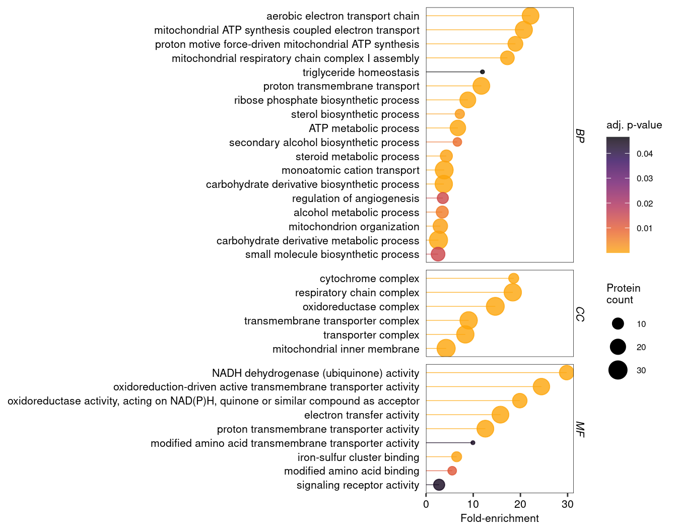
Another useful plot is a dotplot showing the three criticial outcomes of the enrichment analysis: the extent (fold-change) and significance (p-value) of the enrichment, as well as the number of proteins in the target group annotated to a term. However, in the present example we have a total of 312 enriched terms - too many for a useful plot. For GO terms, ClusterProfiler provides the simplify function, which retains only the most significant term for clusters of similar terms.
Code
# Set a theme for ggplot plottingtheme_set( theme( text =element_text(size =8), panel.border =element_rect(linewidth =0.25, colour ="black", fill =NA), panel.background =element_blank(), panel.grid =element_blank(), axis.text =element_text(colour ="black"),strip.background =element_blank(), strip.text =element_text(size =8, face ="italic", vjust =1.1)))# Define a function to simplify an enrichment result object f_simplify_dt <-function(x){ as.data.table( # Return a data.tablesimplify(x, cutoff =0.7 ) # Simplify based on user-defined similarity threshold (default = 0.7) )}# Combine all enrichment results into a single data.tablesimGO_ora_results <-rbind("CC"=f_simplify_dt(oraGO_CC),"BP"=f_simplify_dt(oraGO_BP), "MF"=f_simplify_dt(oraGO_MF), idcol ="Ontology")# Reorder the term description by FoldEnrichmentsimGO_ora_results[, Description :=reorder(Description, FoldEnrichment )]# Make a dotplot using all termspDot <-ggplot( simGO_ora_results, aes(x = FoldEnrichment,y = Description,colour = p.adjust,size = Count))+facet_grid(rows ="Ontology", scales ="free", space ="free")+geom_segment(aes(x =0, xend = FoldEnrichment), linewidth =0.25, show.legend =FALSE)+geom_point()+scale_colour_viridis_c(alpha =0.8, option ="B", direction =-1, end =0.8)+scale_x_continuous(expand =expansion(mult =c(0, 0.05)))+labs(x ="Fold-enrichment", y =NULL, colour ="adj. p-value", size ="Protein\ncount")+theme(axis.ticks.y =element_blank())pDot
Figure 2: Dot plot (or lollipop plot) showing GO term enrichment after removal of redundant terms using the simplify function.
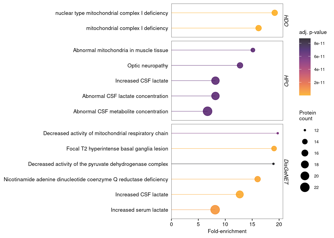
The simplify function works only for GO terms. For disease and phenotype ontologies, removing redundant terms may not be advisable, as it may be relevant to know if the same set of genes is associated with multiple diseases or phenotypes. To simplify such enrichment data, it could be sufficient to filter them based on fold-enrichment and / or p-values.
Code
# Get disease and phenotype ontologies and remove less significant termsdisease_ora_results <- ora_results[ Ontology %in%c("Disease ontology", "Phenotype ontology", "DisGeNET") & p.adjust <1e-10 ]# Reorder the term description by FoldEnrichmentdisease_ora_results[, Description :=reorder(Description, FoldEnrichment )]# Make a dotplot using all termspDot2 <-ggplot( disease_ora_results, aes(x = FoldEnrichment,y = Description,colour = p.adjust,size = Count))+facet_grid(rows ="Ontology", scales ="free", space ="free", labeller =labeller(Ontology =c("Disease ontology"="HDO", "Phenotype ontology"="HPO")))+geom_segment(aes(x =0, xend = FoldEnrichment), linewidth =0.25, show.legend =FALSE)+geom_point()+scale_colour_viridis_c(alpha =0.8, option ="B", direction =-1, end =0.8)+scale_x_continuous(expand =expansion(mult =c(0, 0.05)))+labs(x ="Fold-enrichment", y =NULL, colour ="adj. p-value", size ="Protein\ncount")+theme(axis.ticks.y =element_blank())pDot2
Figure 3: Dot plot showing disease and phenotype enrichments, after removing all terms with an adjusted p-value below 1e-10.
3 Gene Set Enrichment Analysis
GSEA tests for functional enrichment across an entire ranked list of proteins, rather than a predefined “significant” subset. It identifies functional categories that are enriched towards the top (upregulated) or bottom (downregulated) of the ranked list (Subramanian et al. 2005). This approach is particularly useful for detecting subtle, coordinated shifts in protein function that may be missed by ORA.
In ClusterProfiler, GSEA is conducted using functions analogous to those for ORA, but with a key difference in the input. Instead of predefined target and universe lists, the input is a sorted vector where the names are protein IDs and the values are continuous scores, e.g. log2 fold-changes. An alternative ranking metric is the log2 fold-change multiplied by -log10(p-value), taking into account not just the direction and extent of an expression change, but also its significance.
The code below demonstrates how to prepare the input for GSEA and run the analysis for all nine ontologies discussed above. The resulting GSEA output is combined into a single data table for downstream analysis and visualization.
Code
# Create input for GSEA: a sorted, named, numeric vector with unique values.gsea_input <- DT[!duplicated(gene_group) &!is.na(log2_FC_SS6vsSS48) # Remove duplicate genes and NAs ][ order(-log2_FC_SS6vsSS48) # Sort in descending order ][, setNames(log2_FC_SS6vsSS48, gene_group)] # Return named vector # Note: alternatively, one could rank the protein list by (log2-FC * -log10(p-value)), which would take into account both extent *and* significance of expression changes# GSEA - GO - Cellular component (adjust parameters as necessary - see ?gseGO for details)gseaGO_CC <-gseGO(geneList = gsea_input, # Sorted protein list input OrgDb = org.Hs.eg.db, # OrgDb object holding relevant GO data for this specieskeyType ="UNIPROT", # Type of gene ID. Use keytypes(org.Hs.eg.db) to see all optionsont ="CC", # Ontology (BP, CC, MF or ALL)minGSSize =10, # Minimal size of GO termmaxGSSize =500) # Maximal size of GO term# GSEA - BPgseaGO_BP <-gseGO(geneList = gsea_input, OrgDb = org.Hs.eg.db, keyType ="UNIPROT", ont ="BP", minGSSize =10, maxGSSize =500) # GSEA - MFgseaGO_MF <-gseGO(geneList = gsea_input, OrgDb = org.Hs.eg.db, keyType ="UNIPROT", ont ="MF", minGSSize =10, maxGSSize =500) # GSEA - KEGG (only showing non-default options here)gseaKEGG <-gseKEGG(geneList = gsea_input, # Sorted protein list inputorganism ='hsa', # Set organism to human. See ?gseKEGG for more optionskeyType ="uniprot") # Type of protein ID# GSEA - KEGG modules (only showing non-default options here)gseaMKEGG <-gseMKEGG(geneList = gsea_input, # Sorted protein list inputorganism ='hsa', # Set organism to human. See ?gseKEGG for more optionskeyType ="uniprot") # Type of protein ID# For the Reactome GSEA, we require a sorted vector with Entrez IDsentrez_all <-merge(entrez_all, data.table(UNIPROT =names(gsea_input), value = gsea_input), by ="UNIPROT") # Add vevtor values to the Entrez-UniProt mapping tablegsea_input_entrez <- entrez_all[ order(-value) # Sort in descending order ][, setNames(value, ENTREZID)] # Return named vector# GSEA - ReactomegseaRA <-gsePathway(geneList = gsea_input_entrez, # Sorted protein list inputorganism ="human") # Define organism# GSEA - Human disease ontologygseaHDO <-gseDO(geneList = gsea_input_entrez, # Sorted protein list inputont ="HDO") # Specify the disease ontology# GSEA - Human phenotype ontologygseaHPO <-gseDO(geneList = gsea_input_entrez, # Sorted protein list inputont ="HPO") # Specify the phenotype ontology# GSEA - DisGeNETgseaDGN <-gseDGN( geneList = gsea_input_entrez )# Combine all enrichment results into a single data.tablegsea_results <-rbind("Cellular component"=as.data.table(gseaGO_CC),"Biological process"=as.data.table(gseaGO_BP), "Molecular function"=as.data.table(gseaGO_MF), "KEGG"=as.data.table(gseaKEGG),"KEGG module"=as.data.table(gseaMKEGG), "Reactome"=as.data.table(gseaRA), "Disease ontology"=as.data.table(gseaHDO), "Phenotype ontology"=as.data.table(gseaHPO), "DisGeNET"=as.data.table(gseaDGN), idcol ="Ontology")# Show the results as nicely formatted HTML table (DT package)datatable(gsea_results, class =c("display nowrap compact"),rownames =FALSE,options =list(order =list(7, "asc"),paging =FALSE,searching =FALSE,searchHighlight =TRUE,scrollY ="400px", scrollCollapse =TRUE,scrollX =TRUE,fixedHeader =TRUE ) ) %>%formatRound(columns =c("enrichmentScore", "NES"), digits =3) %>%formatSignif(columns =c("pvalue", "p.adjust", "qvalue"), digits =2) %>%formatStyle( "NES",background =styleColorBar(gsea_results$NES, "#c5d4e6"),backgroundSize ='100% 90%',backgroundRepeat ='no-repeat',backgroundPosition ='center') %>%formatStyle( c("Description", "core_enrichment"), overflow ="hidden",textOverflow ="ellipsis",maxWidth ="250px")
Table 2: Combined results of the GSEA analysis for proteins that are significantly change (up- or downregulated) in SS6 cells
Brief explanation of output columns
Ontology: Source of enriched terms
ID: Identifier for GO term, KEGG pathway, etc.
Description: Name of the GO term, KEGG pathway, etc.
setSize: Number of detected proteins annotated to this GO term, KEGG pathway, etc.
enrichmentScore: The degree to which a gene set is overrepresented at the top or bottom of a ranked list. A positive ES indicates gene set enrichment at the top of the ranked list; a negative ES indicates gene set enrichment at the bottom.
NES: Normalized enrichment score; this is the primary statistic for examining GSEA results.
pvalue: Raw p-value for enrichment significance
p.adjust: p-value corrected for multiple testing (BH-adjusted)
qvalue: False discovery rate (similar to p.adjust)
rank: Position in ranked list where maximum enrichment score (ES) was reached. Interesting gene sets achieve the max ES near the top or bottom of the ranked list.
leading_edge: The leading edge subset of a gene set is the subset of members that contribute most to the ES. For a positive ES, the leading edge subset is the set of members that appear in the ranked list prior to the peak score. For a negative ES, it is the set of members that appear subsequent to the peak score. This columns displays the three statistics used to define the leading edge subset. See the GSEA website for more details.
core_enrichment: Proteins that contribute to the leading-edge subset.
3.1 Visualising GSEA results
In GSEA, the magnitude of a term’s enrichment is provided by the normalised enrichment score (NES), which is positive for up- and negative for down-regulated terms. The NES reflects the local concentration of a term along the ranked protein list, capturing whether the genes associated with the term are clustered together. The BH-adjusted p-value (p.adjust) indicates the significance of the enrichment. Importantly, GSEA analyses the entire ranked protein list, allowing significant enrichment (clustering) at any rank position, not just at the very top or very bottom. Therefore, the third critical metric for interpreting GSEA results is the rank: it defines the point of peak enrichment within the ranked data. See the GSEA user guide for more detailed explanations2.
3.2 Exploring GSEA results
To explore GSEA enrichments we plot the NES against term similarity, p-value and rank, respectively.
The advantage of a Manhattan-like plot is that grouping similar terms together facilitates the discovery of unrelated terms, enabling a more systematic exploration of the breadth of the annotations. For GSEA results, the NES can be used on the y-axis instead of the p-value to distinguish between up- and downregulated terms. In addition, since GSEA often assigns the same minimum p-value to multiple terms, its p-values are less suitable for data visualisation.
Code
# Order the ontologiesgsea_results[, Ontology :=factor(Ontology, levels =c("Cellular component", "Biological process", "Molecular function", "KEGG", "KEGG module", "Reactome", "Disease ontology", "Phenotype ontology", "DisGeNET"))]# Create function to define the order of terms within each ontology, grouping similar terms togetherf_term_order <-function(x){ term_similarity =pairwise_termsim(x, showCategory =Inf)@termsim # Map term similarity by Jaccard similarity (without showCategory = Inf the calculation would be truncated at 200 terms) term_distance =as.dist(1-term_similarity) # Turn similarity into a distance metric clustered_terms =hclust(term_distance, method ="ward.D" ) # Cluster terms ordered_terms <-rownames(term_similarity)[clustered_terms$order] # Reorder term names ordered_terms}# Apply this function to order the terms within each ontologygsea_results[, Description :=factor( Description, levels =unique( c(f_term_order(gseaGO_CC),f_term_order(gseaGO_BP),f_term_order(gseaGO_MF),f_term_order(gseaKEGG),f_term_order(gseaMKEGG),f_term_order(gseaRA),f_term_order(gseaHDO),f_term_order(gseaHPO),f_term_order(gseaDGN))) )]# Prepare the data for plotting with Highchartergsea_results <- gsea_results[ order(Ontology, Description), term_index :=1:.N ] # An index for the x-axisgsea_results[, pvalue_sci :=formatC(p.adjust, format ="e", digits =2)] # Format p-values for tooltip gsea_results[, neg_log10_pvalue :=-log10(p.adjust)] # Transform p-value for the y-axis# Create interactive Manhattan plot using Highcharterhchart( gsea_results, "scatter", hcaes(x = term_index, y = NES, group = Ontology)) |>hc_chart( zoomType ="xy") |>hc_xAxis(title =list(text =NULL), # Remove x-axis titlelabels =list(enabled =FALSE), # Remove x-axis labelslineWidth =0.5,lineColor ="black", tickWidth =0 ) |>hc_yAxis( title =list(text ="NES"), lineWidth =0.5, tickWidth =0.5, lineColor ="black", tickColor ="black", gridLineWidth =0 ) |>hc_tooltip(headerFormat ="",pointFormat ="<b>{point.Description}</b> <br>NES: {point.NES:.2f} <br>Adj. p-value: {point.pvalue_sci} <br>Term rank: {point.rank}")
Figure 4: Manhattan-like plot showing all significantly changed gene sets according to GSEA. Terms are grouped by similarity (x-axis). Note the y-axis shows the normalised enrichment score instead of the p-value.
Another way to explore GSEA results is a volcano-like plot, comparing the NES to the p-value:
Figure 5: Volcano-like plot helps to identify the most significantly enriched or depleted gene sets.
A third potentially useful visualisation is the rank of gene sets. Terms with lower rank values peak closer to the top (for positive NES) or closer to the bottom (for negative NES) of the ranked protein list. This could be used to identify terms that are, for example, specifically associated with the most strongly upregulated proteins.
Figure 6: Plot showing the rank of gene sets in the GSEA analysis, compared to their NES. Gene sets (e.g. GO terms) with lower rank values peak closer to the top or bottom of the ranked gene list.
3.3 Simplified GSEA plots
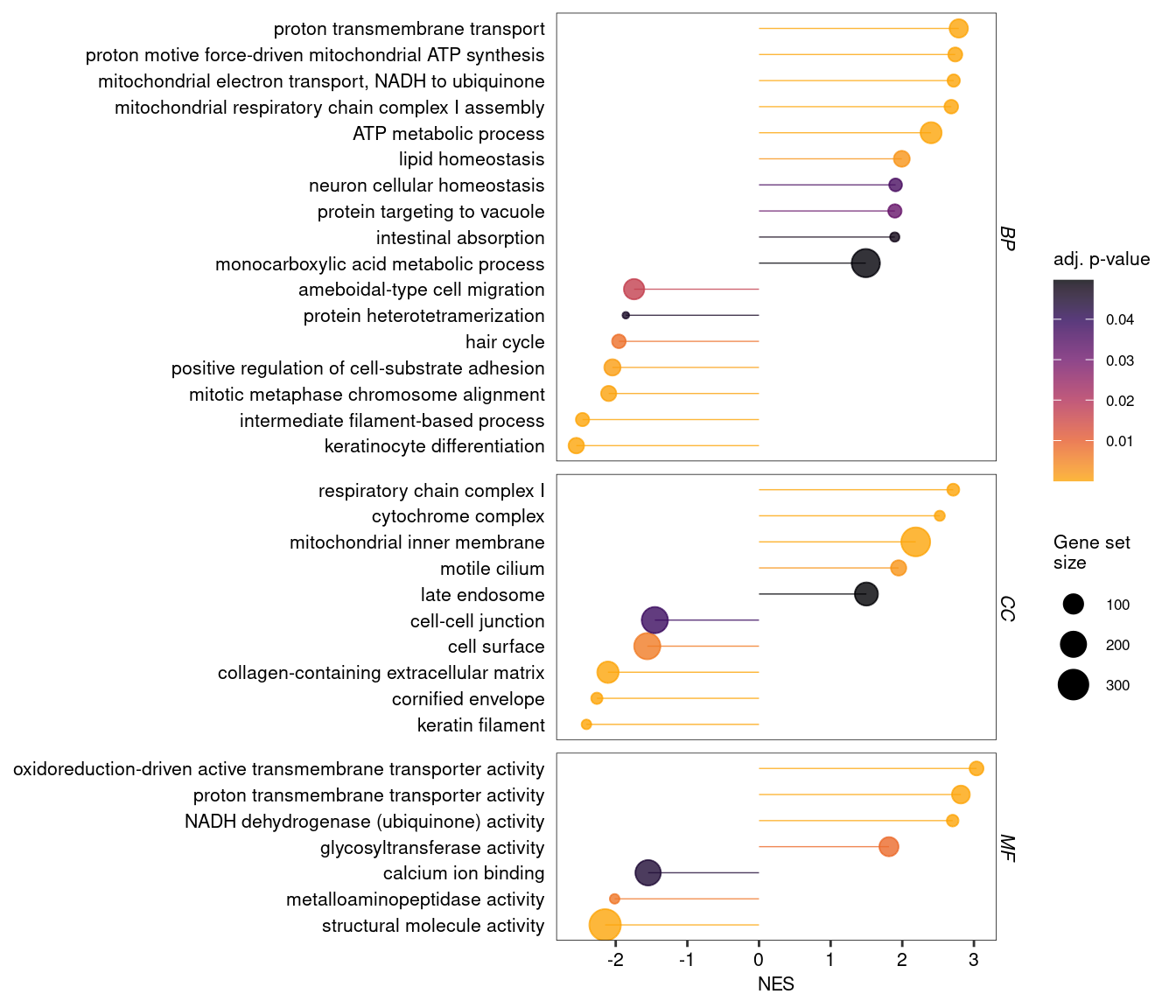
It is also possible to “simplify” GO enrichments from GSEA, in order to visualise a smaller set of non-redundant terms, for example as a dot plot.
Code
# Define a function to simplify an enrichment result object f_simplify_dt <-function(x){ as.data.table( # Return a data.tablesimplify(x, cutoff =0.5 ) # Simplify based on user-defined similarity threshold (default = 0.7) )}# Simplify and combine enrichment results into one data.tablesimGO_gsea_results <-rbind("CC"=f_simplify_dt(gseaGO_CC),"BP"=f_simplify_dt(gseaGO_BP), "MF"=f_simplify_dt(gseaGO_MF), idcol ="Ontology")# Reorder the term descriptionsimGO_gsea_results[, Description :=reorder(Description, NES)]# Make a dotplot using all termspDot <-ggplot( simGO_gsea_results, aes(x = NES,y = Description,colour = p.adjust,size = setSize))+facet_grid("Ontology", scales ="free", space ="free")+geom_segment(aes(x =0, xend = NES), linewidth =0.25, show.legend =FALSE)+geom_point()+scale_colour_viridis_c(alpha =0.8, option ="B", direction =-1, end =0.8)+labs(x ="NES", y =NULL, colour ="adj. p-value", size ="Gene set\nsize")+theme(axis.ticks.y =element_blank())pDot
Figure 7: Dot plot for GSEA-based GO term enrichment, after removal of redundant terms using the simplify function.
3.4 Plotting individual gene sets
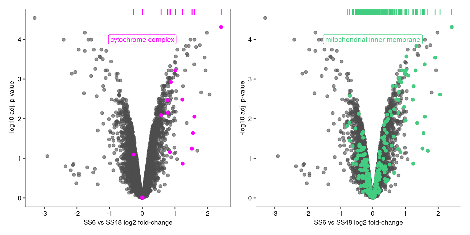
Finally, it can be useful to visualise the distribution of individual, selected gene sets. For example, it may be worth exploring how various GO terms are distributed across the dataset.
For example, the plots below reveal that “cytochrome complex” subunits are consistently among the most upregulated proteins in this datasets, while “mitochondrial inner membrane” proteins are more broadly distributed across the dataset.
Code
# Extract proteins belonging to specific GO terms from the clusterprofiler result objectsterm1 <- gseaGO_CC@geneSets[["GO:0070069"]]term2 <- gseaGO_CC@geneSets[["GO:0005743"]]# Create base plotpVolcano_base <-ggplot(DT, aes( x = log2_FC_SS6vsSS48, y =-log10(adj_p_value)))+geom_point(colour ="grey30", alpha =0.6)+scale_x_continuous(breaks =seq(-4,4,1))+labs(x ="SS6 vs SS48 log2 fold-change", y ="-log10 adj. p-value")# Create plot for first termpTerm1 <- pVolcano_base+geom_point(data = DT[ gene_group %in% term1 ], colour ="magenta")+geom_rug( data = DT[ gene_group %in% term1 ], colour ="magenta", sides ="t" )+annotate("label", x =0, y =4, label = gsea_results[ID =="GO:0070069", Description], colour ="magenta", size =3)# Create plot for second termpTerm2 <- pVolcano_base+geom_point(data = DT[ gene_group %in% term2 ], colour ="seagreen3")+geom_rug( data = DT[ gene_group %in% term2 ], colour ="seagreen3", sides ="t" )+annotate("label", x =0, y =4, label = gsea_results[ID =="GO:0005743", Description], colour ="seagreen3", size =3)# Combine and output plots using patchwork packagepTerm1 + pTerm2
Figure 8: Volcano and rug plots showing the distribution of two GO terms that are both strongly enriched (NES > 2) and highly significant (p.adjust < 1e-9), but have different sizes and distributions.
3.5 Missing sections
In the future, we will also add here:
Function enrichment for other organisms, e.g. Cryptococcus
Comparing multiple conditions at once
References
Baron, J Allen, Claudia Sanchez-Beato Johnson, Michael A Schor, Dustin Olley, Lance Nickel, Victor Felix, James B Munro, et al. 2023. “The DO-KB Knowledgebase: A 20-Year Journey Developing the Disease Open Science Ecosystem.”Nucleic Acids Research 52 (D1): D1305–14. https://doi.org/10.1093/nar/gkad1051.
Gargano, Michael A, Nicolas Matentzoglu, Ben Coleman, Eunice B Addo-Lartey, Anna V Anagnostopoulos, Joel Anderton, Paul Avillach, et al. 2023. “The Human Phenotype Ontology in 2024: Phenotypes Around the World.”Nucleic Acids Research 52 (D1): D1333–46. https://doi.org/10.1093/nar/gkad1005.
Piñero, Janet, Juan Manuel Ramírez-Anguita, Josep Saüch-Pitarch, Francesco Ronzano, Emilio Centeno, Ferran Sanz, and Laura I Furlong. 2019. “The DisGeNET Knowledge Platform for Disease Genomics: 2019 Update.”Nucleic Acids Research, November. https://doi.org/10.1093/nar/gkz1021.
Subramanian, Aravind, Pablo Tamayo, Vamsi K. Mootha, Sayan Mukherjee, Benjamin L. Ebert, Michael A. Gillette, Amanda Paulovich, et al. 2005. “Gene Set Enrichment Analysis: A Knowledge-Based Approach for Interpreting Genome-Wide Expression Profiles.”Proceedings of the National Academy of Sciences 102 (43): 15545–50. https://doi.org/10.1073/pnas.0506580102.
---title: "Functional enrichment analysis"subtitle: "Kustatscher lab tutorial"editor: visualdate: todayformat: htmllink-external-icon: truelink-external-newwindow: trueembed-resources: falsetoc: truenumber-sections: truetheme: light: cosmo dark: superherocode-tools: truecode-fold: truebibliography: references.bib---This vignette provides a reference workflow for functional enrichment analysis, building on our earlier guide for [differential abundance analysis](https://differential-abundance-analysis.netlify.app). We demonstrate how to use the R package [clusterProfiler](https://bioconductor.org/packages/release/bioc/html/clusterProfiler.html) to test protein lists for enrichment of Gene Ontology (GO) terms, as well as other functional and disease-related annotations. The clusterProfiler package is well-documented in manuscripts [@Xu2024; @Wu2021] and other online resources[^1]. Here we demonstrate a clusterProfiler workflow tailored to proteomics data acquired in our lab. The workflow can be adapted to more complex experimental designs.[^1]: ClusterProfiler online resources: - [Complete vignette](https://yulab-smu.top/biomedical-knowledge-mining-book/index.html) - [R package documentation](https://bioconductor.org/packages/release/bioc/manuals/clusterProfiler/man/clusterProfiler.pdf)Functional enrichment analysis can be approached in two main ways:- **Over-Representation Analysis (ORA)**: Identifies functional terms (e.g., GO terms or pathways) that are over-represented in a predefined list of "significant" proteins (e.g. differentially expressed proteins) compared to a background "universe" (e.g. all proteins detected in an experiment). ORA is widely applicable to most experimental designs and is generally straightforward to interpret.- **Gene Set Enrichment Analysis (GSEA)**: Ranks all proteins by a continuous value (e.g. fold-change or p-value) and identifies functional terms that are enriched towards the top or bottom of the ranked list. Unlike ORA, GSEA can detect more subtle, coordinated changes without requiring a hard threshold for "significance." However, it requires an appropriate ranking metric to be available.The statistical principles behind these approaches are described in many online resources, such as this [video series](https://youtu.be/egO7Lt92gDY?feature=shared).::: {.callout-note appearance="minimal"}### How to follow this vignetteCopy the R code chunks and run them locally as you go through this document. You should already be familiar with R data.table and ggplot. The input file `DAA_results.csv.gz` is produced by the [Differential abundance analysis tutorial](https://differential-abundance-analysis.netlify.app). The source code for the whole document is accessible through the Code button in the top right.:::## Preparing the data {#data_prep}As an example, we analyse a simple proteomics experiment that compares protein abundances between two cell lines (SS6 and SS48). We start with a data table containing the log2 fold-changes (e.g. `log2_FC_SS6vsSS48`) and p-values (e.g. `adj_p_value`) derived from a differential protein expression analysis.```{r}#| label: data-and-lib-loading#| message: false# Load the required librarieslibrary(data.table); library(ggplot2); library(highcharter); library(DT); library(clusterProfiler); library(DOSE); library(ReactomePA); library(enrichplot); library(org.Hs.eg.db); library(patchwork)# Load the relevant columns from the differentical expression analysisDT <-fread("DAA_results.csv.gz", select =c("Protein_group", "gene_group", "Genes", "Protein_description", "log2_FC_SS6vsSS48", "adj_p_value"))# Print key columns of this tableDT[ 1:5 , .(Protein_group, gene_group, log2_FC_SS6vsSS48, adj_p_value)]```## Over-Representation AnalysisFor this analysis, we define the target list as proteins upregulated by more than 1.5-fold in the SS6 cell line, with an adjusted p-value \< 0.05 (n = 181). We identify proteins using the `gene_group` column, which contains UniProt gene-level identifiers stripped of isoform annotations. These identifiers are no longer unique, but they are better suited for functional annotation since most annotations are assigned at the gene level rather than the isoform level.Next, we define the background or "protein universe" - the set of proteins against which the target list is compared. The choice of the background is critical for ORA. The entire human proteome (\~20,000 proteins) is often the default background, but it is rarely appropriate. Here we detected 6,332 proteins (corresponding to 6,295 genes), but this set is biased toward abundant proteins, e.g. metabolic enzymes. If we compare our target list against the entire proteome, we risk identifying "enrichment" that simply reflects the bias of proteomics for abundant proteins. Instead, we use the 6,332 detected proteins as our universe. As a general rule, to avoid spurious results ensure that selection biases in the target list also apply to the background list.```{r}#| label: ORA-data-prep# Define the group of proteins to be tested for enrichmenttarget_prots <- DT[ log2_FC_SS6vsSS48 >log2(1.5) & adj_p_value <0.05, gene_group ]# Define the protein universeall_proteins <- DT[, unique(gene_group) ]```### Gene OntologyTesting for GO enrichment is very straightforward in ClusterProfiler. The GO annotation itself is contained in `org.Hs.eg.db`, a Bioconductor genome annotation database, which can be accessed simply by installing the R package with the same name (see section XXXYY for enrichment analysis in other organisms).```{r}#| label: ORA-GO# ORA for GO (adjust parameters as necessary - see ?enrichGO for details)oraGO_CC <-enrichGO(gene = target_prots, # Vector of protein IDs to test (e.g. DEPs)universe = all_proteins, # Vector of protein universe (e.g. all quantified proteins)keyType ="UNIPROT", # Type of protein ID, e.g. UNIPROT, ENSEMBL. Use keytypes(org.Hs.eg.db) to see all optionsOrgDb = org.Hs.eg.db, # OrgDb object holding the relevant GO data for this speciesont ="CC") # Ontology BP, CC, MF or ALL)# We can similarly test for enrichment of biological processes and molecular functionsoraGO_BP <-enrichGO(gene = target_prots, universe = all_proteins, keyType ="UNIPROT", OrgDb = org.Hs.eg.db, ont ="BP") oraGO_MF <-enrichGO(gene = target_prots, universe = all_proteins, keyType ="UNIPROT", OrgDb = org.Hs.eg.db, ont ="MF") ```### KEGGA similar clusterProfiler function can be used to test for enrichment of KEGG pathways and KEGG modules, which are manually defined functional units of genes and reactions.```{r}#| label: ORA-KEGG#| message: false# ORA for KEGGoraKEGG <-enrichKEGG(gene = target_prots, # Vector of protein IDs to test (e.g. DEPs)universe = all_proteins, # Vector of protein universe (e.g. all quantified proteins)organism ='hsa', # Set organism to human. See ?enrichKEGG for more options.keyType ="uniprot") # Type of protein ID# A similar analysis is possible for KEGG modulesoraMKEGG <-enrichMKEGG(gene = target_prots,universe = all_proteins,organism ='hsa',keyType ="uniprot")```### ReactomeClusterProfiler can also perform pathway enrichment analysis using Reactome. However, this functionality requires Entrez IDs instead of UniProt IDs. The ID conversion is straightforward, but it may introduce ambiguous mappings that must be resolved. This typically results in the loss of some proteins. Nevertheless, this conversion step is unavoidable for Reactome pathway analysis, as well as for the subsequent disease and phenotype enrichment analyses. The following code illustrates how to convert UniProt IDs to Entrez IDs and perform the ORA for Reactome pathways.```{r}#| label: ORA-Reactome#| message: false#| warning: false# Convert the protein universe from UniProt to Entrez IDs, using the the bitr functionentrez_all <-data.table(bitr( all_proteins,"UNIPROT", "ENTREZID", OrgDb = org.Hs.eg.db ) ) # Remove ambiguous ID crossmappingsentrez_all <- entrez_all[ !UNIPROT %in% entrez_all[, .N, UNIPROT ][ N >1, UNIPROT ] &# Uniprot IDs matching to more than one Entrez!ENTREZID %in% entrez_all[, .N, ENTREZID][ N >1, ENTREZID ] # Entrez IDs matching to more than one UniProt]# Retrieve the Entrez IDs for the target proteinstarget_prots_ent <- entrez_all[ UNIPROT %in% target_prots, ENTREZID]# Perform ORA for Reactome pathwaysoraRA <-enrichPathway(gene = target_prots_ent, # Vector of protein IDsuniverse = entrez_all$ENTREZID, # Vector of protein universeorganism ="human") # Define organism```### Disease and phenotype ontologiesIn addition to assessing functional enrichment among a set of target proteins, it is also possible to test whether these proteins are enriched for associations with human diseases or phenotypes. ClusterProfiler facilitates this analysis using data from the [Human Disease Ontology](https://disease-ontology.org)[@Baron2024], the [Human Phenotype Ontology](https://hpo.jax.org)[@Gargano2024] and the [DisGeNET](https://disgenet.com) gene-disease association network [@Piñero2020].```{r}#| label: ORA-Disease#| message: false# Test for enrichment of terms from the human disease ontologyoraHDO <-enrichDO(gene = target_prots_ent, # Vector of protein IDs universe = entrez_all$ENTREZID, # Vector of protein universeont ="HDO") # Specify the disease ontology# Test for enrichment of terms from the human phenotype ontologyoraHPO<-enrichDO(gene = target_prots_ent, universe = entrez_all$ENTREZID, ont ="HPO") # Specify the phenotype ontology# Test for enrichment of gene-disease associations from DisGeneNetoraDGN <-enrichDGN(gene = target_prots_ent, # Vector of protein IDsuniverse = entrez_all$ENTREZID) # Vector of protein universe```### Combining ORA resultsAfter running all these enrichment analyses, we can collect their output into a single data table, so we can interpret and visualise the data systematically.```{r}#| label: tbl-ora-output#| tbl-cap: "Combined results of the over-representation analysis for proteins that are significantly upregulated in SS6 cells"# Combine all enrichment results into a single data.tableora_results <-rbind("Cellular component"=as.data.table(oraGO_CC),"Biological process"=as.data.table(oraGO_BP), "Molecular function"=as.data.table(oraGO_MF), "KEGG"=as.data.table(oraKEGG)[, !c("category", "subcategory")], # Remove extra columns added by the enrichKEGG function"KEGG module"=as.data.table(oraMKEGG), "Reactome"=as.data.table(oraRA), "Disease ontology"=as.data.table(oraHDO), "Phenotype ontology"=as.data.table(oraHPO), "DisGeNET"=as.data.table(oraDGN), idcol ="Ontology")# Show the results as nicely formatted HTML table (DT package)datatable(ora_results, class =c("display nowrap compact"),rownames =FALSE,options =list(order =list(6, "desc"),paging =FALSE,searching =FALSE,searchHighlight =TRUE,scrollY ="400px", scrollCollapse =TRUE,scrollX =TRUE,fixedHeader =TRUE ) ) %>%formatRound(columns =c("RichFactor", "FoldEnrichment", "zScore"), digits =3) %>%formatSignif(columns =c("pvalue", "p.adjust", "qvalue"), digits =2) %>%formatStyle( "FoldEnrichment",background =styleColorBar(ora_results$FoldEnrichment, "#c5d4e6"),backgroundSize ='100% 90%',backgroundRepeat ='no-repeat',backgroundPosition ='center') %>%formatStyle( c("Description", "geneID"), overflow ="hidden",textOverflow ="ellipsis",maxWidth ="250px")```::: {.callout-note collapse="true"}### Brief explanation of output columns- Ontology: Source of enriched terms- ID: Identifier for GO term, KEGG pathway, etc.- Description: Name of the GO term, KEGG pathway, etc.- GeneRatio: Proportion of input proteins associated with the term, e.g. 30/180- BgRatio: Proportion of background proteins associated with the term, e.g. 59/6156- RichFactor: Ratio of associated genes in input vs background, e.g. 30/59- FoldEnrichment: Enrichment of term in input vs background, e.g. (30/180) / (59/6156)- zScore: Measure of the significance of deviation from the expected gene count (linked to p-value)- pvalue: Raw p-value for enrichment significance- p.adjust: p-value corrected for multiple testing (BH-adjusted)- qvalue: False discovery rate (similar to p.adjust)- geneID: List of input genes associated with the term- Count: Number of input genes in the term, e.g. 30:::### Visualising ORA resultsEnrichment analyses generally produce redundant results, e.g. identifying multiple, highly similar terms with overlapping gene sets. This makes it difficult to systematically identify the most relevant terms for a particular dataset. There are two options to deal with this:1. **Group Similar Terms**:\ Clustering similar terms into groups allows for a more efficient exploration of the results. This approach is particularly useful during the exploration stage. An effective way to achieve this is by using an interactive, "Manhattan-like" plot, which highlights clusters of similar terms and makes it easier to spot overarching themes in the data.2. **Remove Redundant Terms**:\ Alternatively, redundancy can be reduced by systematically selecting a subset of non-redundant terms, which are then used to create non-interactive, simplified plots for publications or presentations.### Manhattan plots for data explorationAn interactive Manhattan plot, as introduced by [gProfiler](https://biit.cs.ut.ee/gprofiler/page/docs), is an excellent tool for exploring annotations. Terms are grouped by ontology and similarity along the x-axis, so that redundant terms cluster together. This makes it easier to identify distinct, non-overlapping GO terms.```{r}#| label: fig-manhattan-ora#| fig-cap: "A Manhattan-like plot showing all significantly enriched terms. Terms are grouped by similarity."#| fig-height: 4# Order the ontologiesora_results[, Ontology :=factor(Ontology, levels =c("Cellular component", "Biological process", "Molecular function", "KEGG", "KEGG module", "Reactome", "Disease ontology", "Phenotype ontology", "DisGeNET"))]# Create function to define the order of terms within each ontology, grouping similar terms togetherf_term_order <-function(x){ term_similarity =pairwise_termsim(x, showCategory =Inf)@termsim # Map term similarity by Jaccard similarity (without showCategory = Inf the calculation would be truncated at 200 terms) term_distance =as.dist(1-term_similarity) # Turn similarity into a distance metric clustered_terms =hclust(term_distance, method ="ward.D" ) # Cluster terms ordered_terms <-rownames(term_similarity)[clustered_terms$order] # Reorder term names ordered_terms}# Apply this function to order the terms within each ontologyora_results[, Description :=factor( Description, levels =unique( c(f_term_order(oraGO_CC),f_term_order(oraGO_BP),f_term_order(oraGO_MF),f_term_order(oraKEGG),f_term_order(oraMKEGG),f_term_order(oraRA),f_term_order(oraHDO),f_term_order(oraHPO),f_term_order(oraDGN))) )]# Prepare the data for plotting with Highcharterora_results[ order(Ontology, Description), term_index :=1:.N ] # An index for the x-axisora_results[, neg_log10_pvalue :=-log10(p.adjust)] # Transform p-value for the y-axisora_results[, pvalue_sci :=formatC(p.adjust, format ="e", digits =2)] # Format p-values for tooltip # Create interactive Manhattan-like plot using Highcharterhchart( ora_results, "scatter", hcaes(x = term_index, y = neg_log10_pvalue, group = Ontology)) |>hc_chart( zoomType ="xy") |>hc_xAxis(title =list(text =NULL), # Remove x-axis titlelabels =list(enabled =FALSE), # Remove x-axis labelslineWidth =0.5,lineColor ="black", tickWidth =0 ) |>hc_yAxis( title =list(text ="-log10 adj. p-value"), lineWidth =0.5, tickWidth =0.5, lineColor ="black", tickColor ="black", gridLineWidth =0 ) |>hc_tooltip(headerFormat ="",pointFormat ="<b>{point.Description}</b> <br>Fold-enrichment: {point.FoldEnrichment:.2f} <br>p-value: {point.pvalue_sci} <br>Gene count: {point.Count}")```### (Simplified) dot plotsAnother useful plot is a dotplot showing the three criticial outcomes of the enrichment analysis: the extent (fold-change) and significance (p-value) of the enrichment, as well as the number of proteins in the target group annotated to a term. However, in the present example we have a total of 312 enriched terms - too many for a useful plot. For GO terms, ClusterProfiler provides the `simplify` function, which retains only the most significant term for clusters of similar terms.```{r}#| label: fig-dotplot-GO#| fig-cap: "Dot plot (or lollipop plot) showing GO term enrichment after removal of redundant terms using the simplify function."#| fig-height: 5.5#| warning: false# Set a theme for ggplot plottingtheme_set( theme( text =element_text(size =8), panel.border =element_rect(linewidth =0.25, colour ="black", fill =NA), panel.background =element_blank(), panel.grid =element_blank(), axis.text =element_text(colour ="black"),strip.background =element_blank(), strip.text =element_text(size =8, face ="italic", vjust =1.1)))# Define a function to simplify an enrichment result object f_simplify_dt <-function(x){ as.data.table( # Return a data.tablesimplify(x, cutoff =0.7 ) # Simplify based on user-defined similarity threshold (default = 0.7) )}# Combine all enrichment results into a single data.tablesimGO_ora_results <-rbind("CC"=f_simplify_dt(oraGO_CC),"BP"=f_simplify_dt(oraGO_BP), "MF"=f_simplify_dt(oraGO_MF), idcol ="Ontology")# Reorder the term description by FoldEnrichmentsimGO_ora_results[, Description :=reorder(Description, FoldEnrichment )]# Make a dotplot using all termspDot <-ggplot( simGO_ora_results, aes(x = FoldEnrichment,y = Description,colour = p.adjust,size = Count))+facet_grid(rows ="Ontology", scales ="free", space ="free")+geom_segment(aes(x =0, xend = FoldEnrichment), linewidth =0.25, show.legend =FALSE)+geom_point()+scale_colour_viridis_c(alpha =0.8, option ="B", direction =-1, end =0.8)+scale_x_continuous(expand =expansion(mult =c(0, 0.05)))+labs(x ="Fold-enrichment", y =NULL, colour ="adj. p-value", size ="Protein\ncount")+theme(axis.ticks.y =element_blank())pDot```The `simplify` function works only for GO terms. For disease and phenotype ontologies, removing redundant terms may not be advisable, as it may be relevant to know if the same set of genes is associated with multiple diseases or phenotypes. To simplify such enrichment data, it could be sufficient to filter them based on fold-enrichment and / or p-values.```{r}#| label: fig-dotplot-other#| fig-cap: "Dot plot showing disease and phenotype enrichments, after removing all terms with an adjusted p-value below 1e-10."#| warning: false# Get disease and phenotype ontologies and remove less significant termsdisease_ora_results <- ora_results[ Ontology %in%c("Disease ontology", "Phenotype ontology", "DisGeNET") & p.adjust <1e-10 ]# Reorder the term description by FoldEnrichmentdisease_ora_results[, Description :=reorder(Description, FoldEnrichment )]# Make a dotplot using all termspDot2 <-ggplot( disease_ora_results, aes(x = FoldEnrichment,y = Description,colour = p.adjust,size = Count))+facet_grid(rows ="Ontology", scales ="free", space ="free", labeller =labeller(Ontology =c("Disease ontology"="HDO", "Phenotype ontology"="HPO")))+geom_segment(aes(x =0, xend = FoldEnrichment), linewidth =0.25, show.legend =FALSE)+geom_point()+scale_colour_viridis_c(alpha =0.8, option ="B", direction =-1, end =0.8)+scale_x_continuous(expand =expansion(mult =c(0, 0.05)))+labs(x ="Fold-enrichment", y =NULL, colour ="adj. p-value", size ="Protein\ncount")+theme(axis.ticks.y =element_blank())pDot2```## Gene Set Enrichment AnalysisGSEA tests for functional enrichment across an entire ranked list of proteins, rather than a predefined "significant" subset. It identifies functional categories that are enriched towards the top (upregulated) or bottom (downregulated) of the ranked list [@Subramanian2005]. This approach is particularly useful for detecting subtle, coordinated shifts in protein function that may be missed by ORA.In ClusterProfiler, GSEA is conducted using functions analogous to those for ORA, but with a key difference in the input. Instead of predefined target and universe lists, the input is a sorted vector where the names are protein IDs and the values are continuous scores, e.g. log2 fold-changes. An alternative ranking metric is the log2 fold-change multiplied by -log10(p-value), taking into account not just the direction and extent of an expression change, but also its significance.The code below demonstrates how to prepare the input for GSEA and run the analysis for all nine ontologies discussed above. The resulting GSEA output is combined into a single data table for downstream analysis and visualization.```{r}#| label: tbl-GSEA#| tbl-cap: "Combined results of the GSEA analysis for proteins that are significantly change (up- or downregulated) in SS6 cells"#| message: false#| warning: false# Create input for GSEA: a sorted, named, numeric vector with unique values.gsea_input <- DT[!duplicated(gene_group) &!is.na(log2_FC_SS6vsSS48) # Remove duplicate genes and NAs ][ order(-log2_FC_SS6vsSS48) # Sort in descending order ][, setNames(log2_FC_SS6vsSS48, gene_group)] # Return named vector # Note: alternatively, one could rank the protein list by (log2-FC * -log10(p-value)), which would take into account both extent *and* significance of expression changes# GSEA - GO - Cellular component (adjust parameters as necessary - see ?gseGO for details)gseaGO_CC <-gseGO(geneList = gsea_input, # Sorted protein list input OrgDb = org.Hs.eg.db, # OrgDb object holding relevant GO data for this specieskeyType ="UNIPROT", # Type of gene ID. Use keytypes(org.Hs.eg.db) to see all optionsont ="CC", # Ontology (BP, CC, MF or ALL)minGSSize =10, # Minimal size of GO termmaxGSSize =500) # Maximal size of GO term# GSEA - BPgseaGO_BP <-gseGO(geneList = gsea_input, OrgDb = org.Hs.eg.db, keyType ="UNIPROT", ont ="BP", minGSSize =10, maxGSSize =500) # GSEA - MFgseaGO_MF <-gseGO(geneList = gsea_input, OrgDb = org.Hs.eg.db, keyType ="UNIPROT", ont ="MF", minGSSize =10, maxGSSize =500) # GSEA - KEGG (only showing non-default options here)gseaKEGG <-gseKEGG(geneList = gsea_input, # Sorted protein list inputorganism ='hsa', # Set organism to human. See ?gseKEGG for more optionskeyType ="uniprot") # Type of protein ID# GSEA - KEGG modules (only showing non-default options here)gseaMKEGG <-gseMKEGG(geneList = gsea_input, # Sorted protein list inputorganism ='hsa', # Set organism to human. See ?gseKEGG for more optionskeyType ="uniprot") # Type of protein ID# For the Reactome GSEA, we require a sorted vector with Entrez IDsentrez_all <-merge(entrez_all, data.table(UNIPROT =names(gsea_input), value = gsea_input), by ="UNIPROT") # Add vevtor values to the Entrez-UniProt mapping tablegsea_input_entrez <- entrez_all[ order(-value) # Sort in descending order ][, setNames(value, ENTREZID)] # Return named vector# GSEA - ReactomegseaRA <-gsePathway(geneList = gsea_input_entrez, # Sorted protein list inputorganism ="human") # Define organism# GSEA - Human disease ontologygseaHDO <-gseDO(geneList = gsea_input_entrez, # Sorted protein list inputont ="HDO") # Specify the disease ontology# GSEA - Human phenotype ontologygseaHPO <-gseDO(geneList = gsea_input_entrez, # Sorted protein list inputont ="HPO") # Specify the phenotype ontology# GSEA - DisGeNETgseaDGN <-gseDGN( geneList = gsea_input_entrez )# Combine all enrichment results into a single data.tablegsea_results <-rbind("Cellular component"=as.data.table(gseaGO_CC),"Biological process"=as.data.table(gseaGO_BP), "Molecular function"=as.data.table(gseaGO_MF), "KEGG"=as.data.table(gseaKEGG),"KEGG module"=as.data.table(gseaMKEGG), "Reactome"=as.data.table(gseaRA), "Disease ontology"=as.data.table(gseaHDO), "Phenotype ontology"=as.data.table(gseaHPO), "DisGeNET"=as.data.table(gseaDGN), idcol ="Ontology")# Show the results as nicely formatted HTML table (DT package)datatable(gsea_results, class =c("display nowrap compact"),rownames =FALSE,options =list(order =list(7, "asc"),paging =FALSE,searching =FALSE,searchHighlight =TRUE,scrollY ="400px", scrollCollapse =TRUE,scrollX =TRUE,fixedHeader =TRUE ) ) %>%formatRound(columns =c("enrichmentScore", "NES"), digits =3) %>%formatSignif(columns =c("pvalue", "p.adjust", "qvalue"), digits =2) %>%formatStyle( "NES",background =styleColorBar(gsea_results$NES, "#c5d4e6"),backgroundSize ='100% 90%',backgroundRepeat ='no-repeat',backgroundPosition ='center') %>%formatStyle( c("Description", "core_enrichment"), overflow ="hidden",textOverflow ="ellipsis",maxWidth ="250px")```::: {.callout-note collapse="true"}### Brief explanation of output columns- Ontology: Source of enriched terms- ID: Identifier for GO term, KEGG pathway, etc.- Description: Name of the GO term, KEGG pathway, etc.- setSize: Number of detected proteins annotated to this GO term, KEGG pathway, etc.- enrichmentScore: The degree to which a gene set is overrepresented at the top or bottom of a ranked list. A positive ES indicates gene set enrichment at the top of the ranked list; a negative ES indicates gene set enrichment at the bottom.- NES: Normalized enrichment score; this is the primary statistic for examining GSEA results.- pvalue: Raw p-value for enrichment significance- p.adjust: p-value corrected for multiple testing (BH-adjusted)- qvalue: False discovery rate (similar to p.adjust)- rank: Position in ranked list where maximum enrichment score (ES) was reached. Interesting gene sets achieve the max ES near the top or bottom of the ranked list.- leading_edge: The leading edge subset of a gene set is the subset of members that contribute most to the ES. For a positive ES, the leading edge subset is the set of members that appear in the ranked list prior to the peak score. For a negative ES, it is the set of members that appear subsequent to the peak score. This columns displays the three statistics used to define the leading edge subset. See the [GSEA website](https://www.gsea-msigdb.org/gsea/index.jsp) for more details.- core_enrichment: Proteins that contribute to the leading-edge subset.:::### Visualising GSEA resultsIn GSEA, the magnitude of a term's enrichment is provided by the normalised enrichment score (`NES`), which is positive for up- and negative for down-regulated terms. The NES reflects the local concentration of a term along the ranked protein list, capturing whether the genes associated with the term are clustered together. The BH-adjusted p-value (`p.adjust`) indicates the significance of the enrichment. Importantly, GSEA analyses the entire ranked protein list, allowing significant enrichment (clustering) at any rank position, not just at the very top or very bottom. Therefore, the third critical metric for interpreting GSEA results is the `rank`: it defines the point of peak enrichment within the ranked data. See the GSEA user guide for more detailed explanations[^2].[^2]: https://www.gsea-msigdb.org/gsea/doc/GSEAUserGuideFrame.html### Exploring GSEA resultsTo explore GSEA enrichments we plot the NES against term similarity, p-value and rank, respectively.The advantage of a Manhattan-like plot is that grouping similar terms together facilitates the discovery of unrelated terms, enabling a more systematic exploration of the breadth of the annotations. For GSEA results, the NES can be used on the y-axis instead of the p-value to distinguish between up- and downregulated terms. In addition, since GSEA often assigns the same minimum p-value to multiple terms, its p-values are less suitable for data visualisation.```{r}#| label: fig-manhattan-gsea#| fig-cap: "Manhattan-like plot showing all significantly changed gene sets according to GSEA. Terms are grouped by similarity (x-axis). Note the y-axis shows the normalised enrichment score instead of the p-value."#| fig-height: 4# Order the ontologiesgsea_results[, Ontology :=factor(Ontology, levels =c("Cellular component", "Biological process", "Molecular function", "KEGG", "KEGG module", "Reactome", "Disease ontology", "Phenotype ontology", "DisGeNET"))]# Create function to define the order of terms within each ontology, grouping similar terms togetherf_term_order <-function(x){ term_similarity =pairwise_termsim(x, showCategory =Inf)@termsim # Map term similarity by Jaccard similarity (without showCategory = Inf the calculation would be truncated at 200 terms) term_distance =as.dist(1-term_similarity) # Turn similarity into a distance metric clustered_terms =hclust(term_distance, method ="ward.D" ) # Cluster terms ordered_terms <-rownames(term_similarity)[clustered_terms$order] # Reorder term names ordered_terms}# Apply this function to order the terms within each ontologygsea_results[, Description :=factor( Description, levels =unique( c(f_term_order(gseaGO_CC),f_term_order(gseaGO_BP),f_term_order(gseaGO_MF),f_term_order(gseaKEGG),f_term_order(gseaMKEGG),f_term_order(gseaRA),f_term_order(gseaHDO),f_term_order(gseaHPO),f_term_order(gseaDGN))) )]# Prepare the data for plotting with Highchartergsea_results <- gsea_results[ order(Ontology, Description), term_index :=1:.N ] # An index for the x-axisgsea_results[, pvalue_sci :=formatC(p.adjust, format ="e", digits =2)] # Format p-values for tooltip gsea_results[, neg_log10_pvalue :=-log10(p.adjust)] # Transform p-value for the y-axis# Create interactive Manhattan plot using Highcharterhchart( gsea_results, "scatter", hcaes(x = term_index, y = NES, group = Ontology)) |>hc_chart( zoomType ="xy") |>hc_xAxis(title =list(text =NULL), # Remove x-axis titlelabels =list(enabled =FALSE), # Remove x-axis labelslineWidth =0.5,lineColor ="black", tickWidth =0 ) |>hc_yAxis( title =list(text ="NES"), lineWidth =0.5, tickWidth =0.5, lineColor ="black", tickColor ="black", gridLineWidth =0 ) |>hc_tooltip(headerFormat ="",pointFormat ="<b>{point.Description}</b> <br>NES: {point.NES:.2f} <br>Adj. p-value: {point.pvalue_sci} <br>Term rank: {point.rank}")```Another way to explore GSEA results is a volcano-like plot, comparing the NES to the p-value:```{r}#| label: fig-volcanolike-gsea#| fig-cap: "Volcano-like plot helps to identify the most significantly enriched or depleted gene sets."#| fig-height: 4# Create interactive Volcano-like using Highcharterhchart( gsea_results, "scatter", hcaes(x = NES, y = neg_log10_pvalue, group = Ontology)) |>hc_chart( zoomType ="xy") |>hc_xAxis( title =list(text ="NES"), lineWidth =0.5, tickWidth =0.5, lineColor ="black", tickColor ="black", gridLineWidth =0 ) |>hc_yAxis( title =list(text ="-log10 adj. p-value"), lineWidth =0.5, tickWidth =0.5, lineColor ="black", tickColor ="black", gridLineWidth =0 ) |>hc_tooltip(headerFormat ="",pointFormat ="<b>{point.Description}</b> <br>NES: {point.NES:.2f} <br>Adj. p-value: {point.pvalue_sci} <br>Term rank: {point.rank}")```A third potentially useful visualisation is the `rank` of gene sets. Terms with lower rank values peak closer to the top (for positive NES) or closer to the bottom (for negative NES) of the ranked protein list. This could be used to identify terms that are, for example, specifically associated with the most strongly upregulated proteins.```{r}#| label: fig-rankplot-gsea#| fig-cap: "Plot showing the rank of gene sets in the GSEA analysis, compared to their NES. Gene sets (e.g. GO terms) with lower rank values peak closer to the top or bottom of the ranked gene list."#| fig-height: 4# Create interactive Volcano-like using Highcharterhchart( gsea_results, "scatter", hcaes(x = rank, y = NES, group = Ontology)) |>hc_chart( zoomType ="xy") |>hc_xAxis( title =list(text ="Gene set rank"), lineWidth =0.5, tickWidth =0.5, lineColor ="black", tickColor ="black", gridLineWidth =0 ) |>hc_yAxis( title =list(text ="NES"), lineWidth =0.5, tickWidth =0.5, lineColor ="black", tickColor ="black", gridLineWidth =0 ) |>hc_tooltip(headerFormat ="",pointFormat ="<b>{point.Description}</b> <br>NES: {point.NES:.2f} <br>Adj. p-value: {point.pvalue_sci} <br>Term rank: {point.rank}")```### Simplified GSEA plotsIt is also possible to "simplify" GO enrichments from GSEA, in order to visualise a smaller set of non-redundant terms, for example as a dot plot.```{r}#| label: fig-dotplot-GO-gsea#| fig-cap: "Dot plot for GSEA-based GO term enrichment, after removal of redundant terms using the simplify function."#| fig-height: 6# Define a function to simplify an enrichment result object f_simplify_dt <-function(x){ as.data.table( # Return a data.tablesimplify(x, cutoff =0.5 ) # Simplify based on user-defined similarity threshold (default = 0.7) )}# Simplify and combine enrichment results into one data.tablesimGO_gsea_results <-rbind("CC"=f_simplify_dt(gseaGO_CC),"BP"=f_simplify_dt(gseaGO_BP), "MF"=f_simplify_dt(gseaGO_MF), idcol ="Ontology")# Reorder the term descriptionsimGO_gsea_results[, Description :=reorder(Description, NES)]# Make a dotplot using all termspDot <-ggplot( simGO_gsea_results, aes(x = NES,y = Description,colour = p.adjust,size = setSize))+facet_grid("Ontology", scales ="free", space ="free")+geom_segment(aes(x =0, xend = NES), linewidth =0.25, show.legend =FALSE)+geom_point()+scale_colour_viridis_c(alpha =0.8, option ="B", direction =-1, end =0.8)+labs(x ="NES", y =NULL, colour ="adj. p-value", size ="Gene set\nsize")+theme(axis.ticks.y =element_blank())pDot```### Plotting individual gene setsFinally, it can be useful to visualise the distribution of individual, selected gene sets. For example, it may be worth exploring how various GO terms are distributed across the dataset.For example, the plots below reveal that "cytochrome complex" subunits are consistently among the most upregulated proteins in this datasets, while "mitochondrial inner membrane" proteins are more broadly distributed across the dataset.```{r}#| label: fig-volcano-rug-gsea-terms#| fig-cap: "Volcano and rug plots showing the distribution of two GO terms that are both strongly enriched (NES > 2) and highly significant (p.adjust < 1e-9), but have different sizes and distributions."#| fig-height: 4#| fig-width: 8# Extract proteins belonging to specific GO terms from the clusterprofiler result objectsterm1 <- gseaGO_CC@geneSets[["GO:0070069"]]term2 <- gseaGO_CC@geneSets[["GO:0005743"]]# Create base plotpVolcano_base <-ggplot(DT, aes( x = log2_FC_SS6vsSS48, y =-log10(adj_p_value)))+geom_point(colour ="grey30", alpha =0.6)+scale_x_continuous(breaks =seq(-4,4,1))+labs(x ="SS6 vs SS48 log2 fold-change", y ="-log10 adj. p-value")# Create plot for first termpTerm1 <- pVolcano_base+geom_point(data = DT[ gene_group %in% term1 ], colour ="magenta")+geom_rug( data = DT[ gene_group %in% term1 ], colour ="magenta", sides ="t" )+annotate("label", x =0, y =4, label = gsea_results[ID =="GO:0070069", Description], colour ="magenta", size =3)# Create plot for second termpTerm2 <- pVolcano_base+geom_point(data = DT[ gene_group %in% term2 ], colour ="seagreen3")+geom_rug( data = DT[ gene_group %in% term2 ], colour ="seagreen3", sides ="t" )+annotate("label", x =0, y =4, label = gsea_results[ID =="GO:0005743", Description], colour ="seagreen3", size =3)# Combine and output plots using patchwork packagepTerm1 + pTerm2```### Missing sectionsIn the future, we will also add here:- Function enrichment for other organisms, e.g. Cryptococcus- Comparing multiple conditions at once